Conditional Formatting using Countifs - helpClosed

Question

=COUNTIFS(D$3:D$21,"Yes",$A$3:$A$21,$A3)>1
Above is my countif statement to count the number of times a particular criteria exists.

D3:D21 should be 'Yes' and A3:A21 should contain the value in A3. The conditional formatting works for A3 and A9 where D3 and D9 is "Yes". However, in A18, when the value is same as the value in A3 and D18 is "No", the field is still formatted as above. 

How do I get it to format only if D3:D21 is a 'Yes' and the value ins A3:A21 is the same as value in A3?

Mazzaropi · Answer

prady3011, Good morning. 

I'm not sure if I understood well your necessity.

Try to use:

=AND(COUNTIFS($D$3:$D$21,"Yes",$A$3:$A$21,$A$3)>1 , $A3="YES")

Is it what you want?
I hope it helps.

prady3011 · Answer

Hi Mazzaropi,
I've got the following data in column A and column D. I want to conditionally format Column D, where the value in Column A is 'a' and the value in Column D is 'Yes'. However, with my current formula, mentioned above, Column D is being formatted even when the value in it is 'No' (see last line of the the data)

So, what I want to do is: the cells to be highlighted for every value in column A, where Column D is a 'Yes' and this combination occurs more than once.
In example below: I want the following cells to be highlighted where A = a and D =Yes and it occurs more than once. In the example, the combination occurs twice - and I want to conditionally format it, but with my formula even the cell where A = a and D = No is being highlighted.

Your formula, doesn't highlight anything.

A      D
a	Yes
b	0
c	0
v	0
Music Team	
a	Yes
f	0
v	0
c	0
YPS Team	
a1	0
b1	0
c1	0
d1	0
Communion Team	
a	No

Mazzaropi · Answer

prady3011, Good afternoon.

I did an Excel file to show you the formula I mentioned before using your data as example.
Please, take a look at it.
http://speedy.sh/3WYfz/04-11-2014-en-Kioskea-Conditional-Formatting-OK.xlsx

Is it what you want?
I hope it helps. 
 --
Belo Horizonte, Brasil.
Marcílio Lobão

prady3011 · Answer

Hi Marcilio,
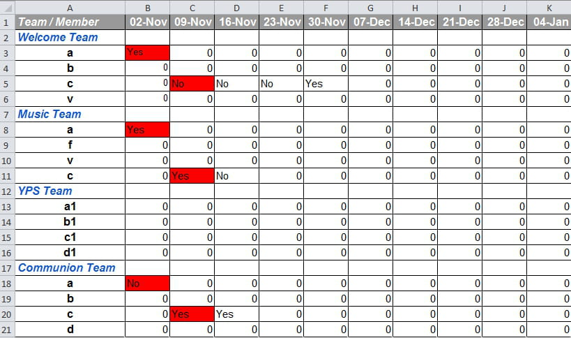
You're attachment was quite helpful, but not exactly what I want. I've attached an image below. You're formula works only when the value in column A is 'a', but I want it to apply to value 'c' , etc.

I want the cells to be highlighted only for the following combinations:
If the value is Yes, for any value in column A and if the value in Column A repeats more than once, the cell should be hightlighted. In my image, I don't want 'No' to be highlighted.

Thanks for your help so far.

Mazzaropi · Answer

prady3011, Good afternoon.

"...If the value is Yes, for any value in column A and if the value in Column A repeats more than once, the cell should be hightlighted. In my image, I don't want 'No' to be highlighted..."

Take a look at it:
http://speedy.sh/bcm2E/04-11-2014-en-Kioskea-Conditional-Formatting-OK.xlsx

Please, tell us if it worked for you.
I hope it helps. 
 --
Belo Horizonte, Brasil.
Marcílio Lobão

Conditional Formatting using Countifs - help

5 responses

Similar discussions

Subscribe To Our Newsletter!