
Conditional Formatting: Font color for entire column based on another column
Solved/Closed
Kitkatpdx
Posts
3
Registration date
Tuesday January 12, 2021
Status
Member
Last seen
January 13, 2021
-
Jan 12, 2021 at 09:49 PM
Mazzaropi Posts 1983 Registration date Monday August 16, 2010 Status Contributor Last seen May 24, 2023 - Jan 13, 2021 at 01:04 PM
Mazzaropi Posts 1983 Registration date Monday August 16, 2010 Status Contributor Last seen May 24, 2023 - Jan 13, 2021 at 01:04 PM
Related:
- Conditional formatting excel column based on another column
- Excel column number - Guide
- Excel conditional formatting based on date - Guide
- Excel clear formatting - Guide
- Excel conditional formatting based on text ✓ - Excel Forum
- Excel conditional formatting based on another cell - Excel Forum
3 responses
Mazzaropi
Posts
1983
Registration date
Monday August 16, 2010
Status
Contributor
Last seen
May 24, 2023
147
Jan 13, 2021 at 12:33 PM
Jan 13, 2021 at 12:33 PM
KItKatpdx, Good afternoon.
Try to do this one:
Select the range you desire: ex.: A3:A50
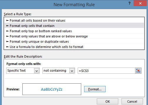
Menu --> Conditional Format --> New rule
1) Use a formula to determine which cells to format:
Use the formula: =B3<>""
Format Font color as you want: BLUE -- OK
New rule
2) Use a formula to determine which cells to format:
Use the formula: =C3<>""
Format Font color as you want: RED -- OK
OK
Please, tell us if it worked for you.
I hope it helps.
Try to do this one:
Select the range you desire: ex.: A3:A50
Menu --> Conditional Format --> New rule
1) Use a formula to determine which cells to format:
Use the formula: =B3<>""
Format Font color as you want: BLUE -- OK
New rule
2) Use a formula to determine which cells to format:
Use the formula: =C3<>""
Format Font color as you want: RED -- OK
OK
Please, tell us if it worked for you.
I hope it helps.

Jan 13, 2021 at 12:35 PM