Conditional Formatting: 3 range of numbers

Solved/Closed

LCC - May 5, 2015 at 09:36 PM
LCC - May 10, 2015 at 11:01 PM

Hello,

would like to seek advice from some of the experts here.

I want to do conditional formatting from column O6-O21.

If percentage is above 100%, cell will be green filled with black font

If percentage between 80-100%, cell will be yellow filled with black font

If percentage is below 80%, cell will be red filled with black font

anyone can help?

THANK YOU!

Excel conditional formatting 3 color scale formula
Conditional formatting 3 color scale percentages - Best answers
Conditional formatting excel 3 color scale formula - Best answers
Hitman 3 cheats - Guide
Psiphon 3 download - Download - VPN
Excel conditional formatting if another cell contains specific text ✓ - Excel Forum
Position formula in excel ✓ - Office Software Forum
Excel conditional formatting if cell contains specific text - Excel Forum

1 response

Answer 1 / 1

MaxStart Posts 339 Registration date Tuesday March 3, 2015 Status Moderator Last seen July 3, 2015 69
May 8, 2015 at 07:40 AM

Hi there ..

Select your range

Right Click and set format as percentage

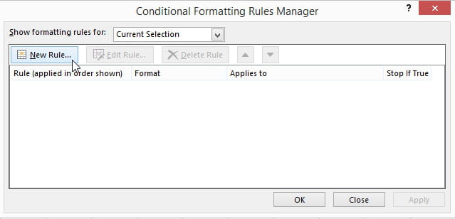
Go to: Conditional Formatting -> Manage Rules:

1- New Rule

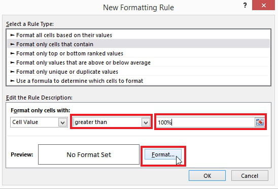
2- Choose: Format only cells that contain:

for the first rule choose: Grater than, enter the value and choose the formatting you need:

for the second rule repeat the steps 1 + 2 then choose: Value Between:

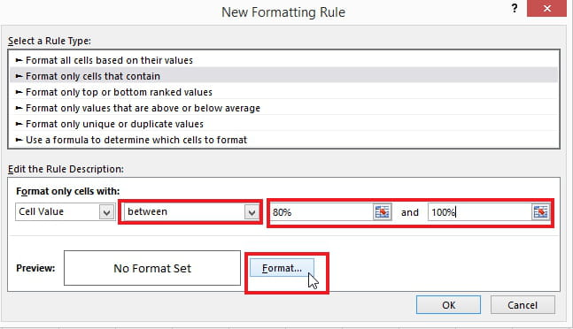
Create the Last Rule and hit OK

Result

Good Luck

LCC
May 10, 2015 at 11:01 PM

Thanks a lot! Tried it and it works! appreciate your time and effort to answer! Cheers!

Similar discussions

Conditional Formatting (more than 3) in Excel

How to use conditional format based on text?

Conditional Formatting: Font color for entire column based on another column

conditional formatting on multiple criteria

Conditional format based on another cell containing text

Condition formatting on changing cell color based on another cel

Result

Similar discussions

Subscribe To Our Newsletter!