Cell format
Solved/Closed
mastachaah
Posts
2
Registration date
Sunday March 15, 2015
Status
Member
Last seen
March 17, 2015
-
Mar 16, 2015 at 02:25 AM
MaxStart Posts 338 Registration date Tuesday March 3, 2015 Status Moderator Last seen July 3, 2015 - Mar 17, 2015 at 12:13 PM
MaxStart Posts 338 Registration date Tuesday March 3, 2015 Status Moderator Last seen July 3, 2015 - Mar 17, 2015 at 12:13 PM
Related:
- Cell format
- Dvi format - Guide
- Kingston format utility - Download - Storage
- Format usb ubuntu - Guide
- Hp usb disk storage format tool - Download - Storage
- Hdd low level format tool - Download - Storage
1 response

MaxStart
Posts
338
Registration date
Tuesday March 3, 2015
Status
Moderator
Last seen
July 3, 2015
69
Mar 16, 2015 at 10:23 PM
Mar 16, 2015 at 10:23 PM
OK, the answer to your issue is Conditional formatting
I've made an example for you
Cell A1 will contain the drop-down list witch contains the following
%
RM
Date
now Cell B1 will change format according to cell A1 value
just write anything in cell B1 to see resauts
1- go to Conditional formatting and choose new rule
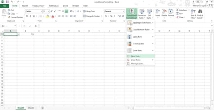
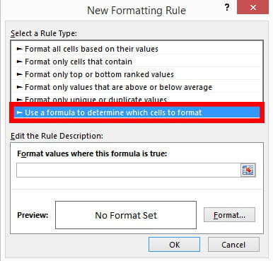
2- now you need to select the drop-down litst cell entering the following formula
=$A$1="%"
3- now go to the format button and choose the percentage format and maybe change the fill color for differentiation.
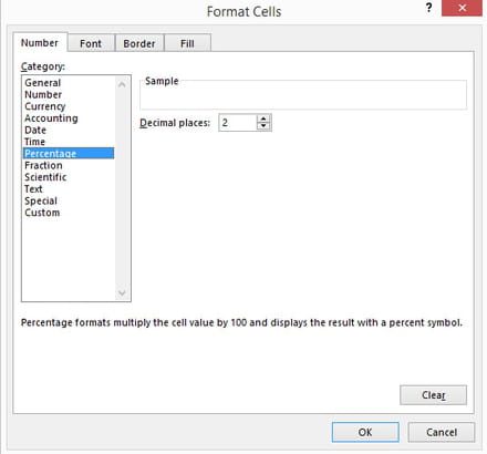
4- click ok.
5- repeat steps from 1 to 4 for each value in the drop-down list just change the conditions accordingly
=$A$1="%"
=$A$1="RM"
=$A$1="Date"
6- now go to conditional formatting and choose manage rules
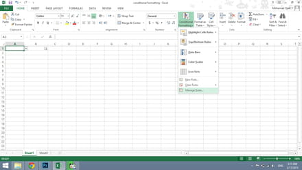
7- change the targeting rules accordingly
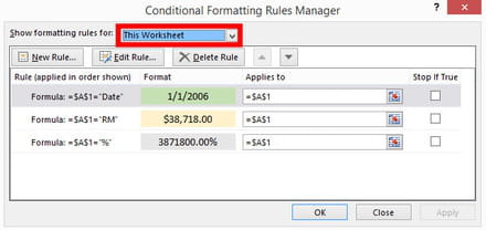
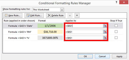
this should work just fine.
feed us back if it woks for you.
I've made an example for you
Cell A1 will contain the drop-down list witch contains the following
%
RM
Date
now Cell B1 will change format according to cell A1 value
just write anything in cell B1 to see resauts
1- go to Conditional formatting and choose new rule


2- now you need to select the drop-down litst cell entering the following formula
=$A$1="%"
3- now go to the format button and choose the percentage format and maybe change the fill color for differentiation.

4- click ok.
5- repeat steps from 1 to 4 for each value in the drop-down list just change the conditions accordingly
=$A$1="%"
=$A$1="RM"
=$A$1="Date"
6- now go to conditional formatting and choose manage rules

7- change the targeting rules accordingly


this should work just fine.
feed us back if it woks for you.


Mar 17, 2015 at 11:37 AM
Mar 17, 2015 at 12:13 PM
just make thee Decimal places = 0